| Overview |  |
Copyright © Quviq AB, 2006-2025
Version: 1.48.3
This module is designed for testing software with a finite number of abstract states--for example software described by UML statecharts. It allows users to specify a collection of named states and the transitions between them, along with pre- and post-conditions and state transition functions. Users can assign weights to transitions, to achieve a good statistical distribution of test cases, and eqc_fsm can help users do so by generating visualizations of the state diagram, and by automated weight assignment.
eqc_fsm is closely related to eqc_statem, and
generates test cases of precisely the same form. (One way to think
of eqc_fsm is that it is to eqc_statem as
gen_fsm is to gen_server). We assume that readers
are already familiar with eqc_statem; if not, study the
eqc_statem documentation before reading further.
The cases in which you may prefer eqc_fsm over eqc_statem
are when you have a test API for which some API calls are clearly
only callable when the Software Under Test is in a specific state.
This situation can be solved by adding preconditions to the eqc_statem
QuickCheck model, but alternatively, can be handled using the eqc_fsm
modeling approach.
Since release 1.35 of QuickCheck, the documentation of this module has been updated to the grouped style of writing callbacks. In case you are confronted with a legacy state machine model that you need to understand, please read the old documentation.
The examples directory distributed with QuickCheck contains a module lock_eqc.erl (source code) that illustrates how eqc_fsm can be used in a simple case.
State machines are specified by a module defining callback
functions that are invoked to test the state machine. The
callbacks closely resemble those used by eqc_statem.
The main differences
are the addition of a finite state machine to specify when
certain commands can be generated. A collection of functions
corresponding to named states specify in what state a certain
command can be added to a test case.
The other difference is that callbacks have two more arguments:
a From state and a To state.
-include_lib("eqc/include/eqc_fsm.hrl"). (If QuickCheck is not installed in your Erlang library directory, then you will need to use -include and give a different path). This imports all the exported functions from eqc_fsm, together with those functions from eqc_statem that are usable with eqc_fsm too. Note that you should not include eqc_statem.hrl in the same module.
eqc_fsm tracks the state of each test case, just as
eqc_statem does, but eqc_fsm splits the state into
two parts: a state name (normally an atom), which
corresponds to one of the states in a finite-state machine diagram,
and state data, which may be any relevant information, but
is normally a record. This is a similar distinction to that made
between state names and state data by gen_fsm in the OTP
libraries. Complete states are represented by a pair of the state
name and the state data.
Each named state is defined by a function of the same name, which returns a list of target state names to which a transition can be made, paired with function calls whose execution follows that transition. For example, in a system with two named states, locked and unlocked, the unlocked state might be specified by
  unlocked(S) ->
    [{unlocked,read}},
     {locked,  lock}].
which specifies that a transition from the unlocked state to the locked state can be made by calling the lock function, or we can call the read function and remain in the same state. eqc_fsm generates test cases which follow the transitions specified in this way from state to state. The argument generators for the lock and read function are generated with an _args callback in the same way as eqc_statem provides argument generation.
If the target state name is the atom history, then this represents a transition to the same state. This can be used to abstract a set of transitions that can be used in several different states. For example,
  read_transition() ->
    [{history, read}].
could be used to define a read transition that can be included in any other state by adding read_transition()++... to the state definition; whatever state it is used in, the read transition returns to the same state.
State functions may take additional parameters, called attributes. For example,
  unlocked(N) ->
    [{{unlocked,N+1}, add} || N<4] ++
    [...other transitions...].
might represent a locker containing N values. When attributes are used, then the state names are tuples of the function name and the attribute values. States with different attribute values are considered to be different states: {unlocked,0} and {unlocked,1} are different states in this example. Since QuickCheck enumerates every reachable state, then it is important that there are only finitely many reachable attribute values--this is why we only include an add transition when N is less than 4 in the example above--this ensures that states {unlocked,N} are not reachable for N greater than or equal to 5.
It is perfectly allowable for the list of transitions to depend on the values of attributes, as in this example.
This symbolic state is evaluated to construct the initial dynamic state before each test case is executed.
The following callback suffixes are provided for eqc_fsm.
state_data()) :: bool()
Returns true if the command COMMAND may be generated in state S. The precondition is also used when shrinking to make sure that invalid commands do not pop-up in a test case while shrinking. Note that there is a subtle difference between preconditions in eqc_fsm compared to eqc_statem. In eqc_fsm a precondition that raises an exception is assumed to be false.
default: truestate_data(), Args::[term()]) :: bool()
Returns true if the symbolic call {call,_,COMMAND,Args} can be performed in the state S. The precondition is also used when shrinking to make sure that invalid commands do not pop-up in a test case while shrinking.
default: true
Preconditions are used to decide whether or not to include candidate commands in test cases, which is why only the symbolic state information is available when preconditions are checked.
state_data()) :: eqc_gen:gen([term()])
Generates appropriate arguments for the function under test. The result are arguments Args that are used in the symbolic call
{call,?MODULE,COMMAND,Args} in the test case generator, given that COMMAND_pre(S)
returns true for the symbolic state S at generation time.
This is the function that is called during test case execution.
state_data(), V::var(), Args::[term()]) :: state_data()
This is the state transition function of the abstract state machine, and it is used during both test generation and test execution. The type above refers to calls during test generation.
In this case, it computes the symbolic state after symbolic call {call,_,COMMAND,Args}, performed in symbolic state S, with result V. Because it is applied to symbolic states and symbolic calls, the result of the call must also be symbolic-- in fact, V is the symbolic variable which will be set to the result of the call.
For example, if the state were a list of pids, and COMMAND applied to Args spawned a new process, then the variable V could be added to the state to refer to the pid of the process just spawned. Symbolic function calls can also be included in the next state, to construct parts whose values will only be known during test execution.
The same function is used to compute the next dynamic state during test execution. In this case S is the previous dynamic state, and Args are the actual values passed (not symbolic argument expressions), and V is the actual value returned--in other words, all the symbolic inputs are replaced by their values. A correctly written COMMAND_next function does not inspect symbolic inputs--it just includes them as symbolic parts of the result. Thus the same code can construct a dynamic state of the same shape, given actual values instead of symbolic ones. The only difficulty is that COMMAND_next may itself introduce symbolic function calls into its result, which would then be a kind of mixture of a symbolic and dynamic state. To ensure that the state remains dynamic during test execution, any such symbolic calls are performed, and replaced by their values, before test execution continues.
default: S, i.e., leave state unchangeddynamic_state(), Args::[term()], R::term()) :: bool()
Checks the postcondition of symbolic call {call,_,COMMAND,Args}, executed in dynamic state S, with result R.
default: trueOf course, postconditions are checked during test execution, not test generation.
An important special case is checking that the result of COMMAND matches the expected return value. If COMMAND_return is specified this is done by:COMMAND_post(From :: state_name(), To :: state_name(), S, Args, Res) -> eq(Res, COMMAND_return(S, Args)).
state_data(), Args::[term()]) :: term()
This is an optional callback that computes the expected return value from the model state. This return value can be used in simulation mode, or when clustering a state machine with a component. It is often good practice to check the return value in the postcondition by explicitely calling this return callback to check whether the actual returned value is equivalent with the return value computed by this function using the model state.
The return function can be an over specification, not leaving enough implementation freedom. In those cases it is preferred to use a general postcondition, which might check that the returned value is in a certain range or of a certain form.
dynamic_state(), Args::[term()], R::term()) :: list(any())
Collects a list of features of the symbolic call {call,_,COMMAND,Args}, executed in dynamic
state S, with result R.
The arguments of the symbolic call are the
actual values passed, not any symbolic expressions from which they were computed.
The features can be recovered later using call_features/1.
Features are collected during test execution, not test generation.
dynamic_state(), Args::[term()]) :: bool()
This is an optional callback which can be used to check a precondition during test execution. Its argument is a dynamic state, and a call with the actual argument values (even for calls which are generated with symbolic arguments). If it returns false, then the command is not executed during the test. Dynamic preconditions may be easier to write than the normal preconditions, because they need not work with symbolic values. However, they have significant disadvantages:
parallel_commands/1 is not possible.
For these reasons, it is almost always better to enrich the model state so that a static precondition can be defined, than to use a dynamic one. In rare cases, and especially when the dynamic precondition will usually be true, then using this callback can be the best approach.
default: trueThis is an optional callback which specifies the distribution with which commands are generated. Commands are normally generated with a uniform distribution, unless a weight function is provided. In this case the weight computed from the command is used as frequency.
This is an optional callback which specifies the priority with with a transition is chosen. Default priority is one, higher priority makes it more likely that a transition chosen in a generated test case.
dynamic_state()) :: bool()
This is an optional callback which can be used to check an invariant during test execution. It is called at the beginning of each command sequence with the initial state as argument, and then after each command is executed with the resulting state as argument. Its second argument is always a dynamic state; it is not used during test case generation. If invariant returns anything other than true, the test fails. Its intended use is to compare the model state S with the actual state of the system under test.
If invariant is not defined by the user, then it is assumed to be true.
precondition_common(From :: state_name(), To :: state_name(), S::state_data(), Call::[call()]) :: bool()
Used to specify a general precondition. This precondition is applied after command generation, but before the specific (COMMAND_pre/4. Thus in COMMAND_pre/4 one may assume that the general precondition holds.
command_precondition_common(From :: state_name(), To :: state_name(), S::state_data(), COMMAND :: atom()) :: bool()
command_precondition_common(S, Cmd) ->
    S /= uninitialized orelse Cmd == init.
This precondition ensures that unless the state is not uninitialized the
command must be init.
postcondition_common(From :: state_name(), To :: state_name(), S::state_data(), Call::[call()], Res::term()) :: bool()
eqc_component is to check that all return values follow what we expect:
postcondition_common(S, Call, Res) ->
    eq(Res, return_value(S, Call)).
call_features_common(From :: state_name(), To :: state_name(), S::state_data(), Call::[call()], Res::term()) :: bool()
eqc_fsm specifications are tested using very similar
properties to eqc_statem specifications: the only
difference is that the commands/1 and
run_commands/2 functions are imported from eqc_fsm
instead (which is done by the eqc_fsm.hrl include
file). Thus a suitable propery might look something like this:
  prop_locker() ->
    ?FORALL(Cmds,commands(?MODULE),
      begin
        locker:start(),
        {H,S,Res} = run_commands(Cmds),
        locker:stop(),
        Res == ok
      end).
The definitions of state functions described above offer no opportunity to specify how often each transition should be chosen. This is done instead by a separate callback:
weight(From, To, Cmd, Args) -> integer()
This callback is optional: if it is omitted (or not
exported), then the transitions from each state are chosen with
equal probability. If weight is defined, then the weights
it assigns to each transition are used in the same way as the
weights passed to the eqc_gen:frequency/1 function: the
probability of choosing a transition is proportional to the weight
assigned to it.
It is important to measure the resulting distribution of transitions in the generated test data. This can be done during testing by amending the last line of the property above to
  aggregate(zip(state_names(H), command_names(Cmds)),
            Res == ok)
using the functions eqc:aggregate/2, state_names/1,
eqc_statem:command_names/1, and
eqc_statem:zip/2. The output generated shows the proportion
of each state name/function name combination in the total set of
transitions run.
eqc_fsm can generate diagrams visualizing the state space and the transitions between states, along with the frequency with which each transition is tested.
QuickCheck uses external tools to generate and display visualizations. Users need to install these tools separately, and make them available to QuickCheck.
QuickCheck generates visualizations of the state space in the dot graph description language. These can be converted to a wide variety of image formats using the GraphViz tools, which can be downloaded from www.graphviz.org for a wide variety of platforms, under the open-source Common Public Licence.
Once installed on your system, ensure that dot (or dot.exe) is accessible via your path. If you can invoke dot in your shell by typing dot, then QuickCheck should be able to make use of it. Alternatively, you can specify the location of this file in the environment variable EQC_DOT. QuickCheck will use dot to generate JPEG visualizations (or another supported image type of your choice).
If you provide QuickCheck with a JPEG viewer, then it will use it to display visualizations automatically. Under Windows XP and Vista, nothing needs to be done--your default JPEG viewer will be used automatically. Under other operating systems (or if you want to use a different viewer), you should set the environment variable EQC_VIEWER to the location of the viewer of your choice. QuickCheck displays images by running a shell command of the form <EQC_VIEWER> <filename>.jpg. You can specify another image type supported by GraphViz when generating images; in this case, the viewer should of course be suitable for the type of image you choose.
Visualizations are created and displayed by visualize/1. If
only the dot file is required, then it can be generated by dot/1. The visualizations include the estimated frequency of each
transition when tests are run, such as this
example:
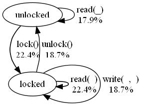
The percentages shown are the number of times the labelled transition will be followed during testing, as a percentage of the total number of transitions followed. The result of the analysis should agree with measured transition frequencies when sufficiently any tests are run (several thousands)--but the analysis is much quicker.
The results can be used to help assign appropriate weights to transitions. Users should aim to avoid orphan transitions, which are tested very rarely, because bugs which depend on such orphans will take a very long time to find.
QuickCheck can predict the frequency with which each transition in the state machine will be followed during testing, and can also use these predictions to suggest a suitable choice of weights.
The analysis assumes that once a transition has been chosen, then a suitable call can always be generated. If attempts to generate a call can fail--either because the generation raises an exception, or because the precondition is false--then the analysis will overestimate the frequency of that and subsequent transitions. It is important to compare the analysis results with actual measured transition frequencies, to see to what extent this is occuring.
To perform an accurate analysis, QuickCheck needs to know how often the attempt to generate a suitable call fails--which cannot be determined in advance. Users can provide an estimate of this by defining the (optional) callback _preprobability The result should be a float between 0 and 1, which is the estimated probability of succeeding to generate a call satisfying the precondition for this transition. For example, if we expect generation of a read call in an unlocked state to fail half the time, then we could define
  read_preprobability(unlocked, _, [_]) -> 0.5;
  read_preprobability(_, _, _) -> 1.0.
QuickCheck can assign weights to transitions automatically, taking into account the user's estimates of precondition probabilities specified above. QuickCheck compensates for a low precondition probability by trying to choose that transition more often. Weights are assigned so as to avoid orphan transitions, as far as possible--although in most cases, no assignment of weights can ensure an absolutely even distribution of testing effort.
The weight assignment is computed by automate_weights/1,
which outputs a candidate definition of the weight callback, and
(if GraphViz and a JPEG viewer are available) visualizes the
resulting transition frequencies. The definition of weight
can be pasted back into the eqc_fsm specification, to
cause QuickCheck to use the computed weights.
The assigned weights are not necessarily "optimal" in any sense, but are often better than a hand-assignment. It is still important to measure actual transition distribution, and tune the assigned weights if necessary.
Often, some transitions should be tested more often than others: for example, one transition may call a function with no arguments, while another may have many complex arguments, with a wide variety of choices to explore. Of course, the latter needs to be tested more often than the former. When weights are assigned manually, then the user can take this into account by weighting the latter transition more highly, but when they are assigned automatically then a different mechanism is required.
Users can prioritize transitions by defining the optional callback
priority(From, To, Cmd, Args) -> integer() | float()with the same parameters as
precondition_probability. The
automated weight assignment will then choose weights that increase
the execution frequency of highly prioritized transitions. For
example, using the same state machine as in the diagram above, we
could increase the priority of lock transitions by defining
  priority(unlocked,_,lock,_) -> 10;
  priority(_,_,_,_) -> 1.
The resulting transition frequencies are as shown here:
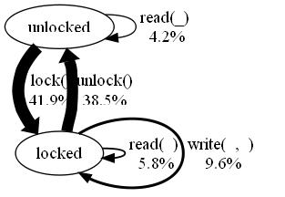
Note that both the lock and unlock transitions are
assigned a greater weight--the latter, because choosing unlock is
necessary to permit another lock, so unlocking more often permits
more tests of locking. Automated weight assignment takes into
account these kinds of interactions between transitions, which is
hard to do well by hand.
-eqc_fsm(external_fsm).one can specify the state transition functions outside the actual callback module in a different module with same name as callback module and extension .fsm. This is useful when using a graphical editor to manipulate the state machine representation.
callback_module() = atom()
The name of a module containing the eqc_fsm callbacks, as specified above.
abstract datatype: command()
Command type defined by eqc_statem:command().
abstract datatype: dynamic_state()
The type used by the callback module to represent
the state of a test case during test execution. It is the same as
eqc_statem:symbolic_state(), except that symbolic variables and calls
are replaced by their values.
flows() = [{float(), transition_pattern()}]
A list of transition patterns, paired with the proportion of executed transitions that match that pattern. The proportions sum to 1.
abstract datatype: gen(A)
QuickCheck generator type defined by eqc_gen:gen().
abstract datatype: history()
State machine history type defined by eqc_statem:history().
abstract datatype: parallel_test_case()
Type defined by eqc_statem:parallel_test_case().
pattern() = any()
A term possibly containing the atom '_', which matches any similar term where occurrences of '_' may match any value.
abstract datatype: reason()
Type defined by eqc_statem:reason().
state_data() = any()
state_name() = atom() | tuple()
abstract datatype: symbolic_state()
Type defined by eqc_statem:symbolic_state().
transition_pattern() = {state_name(), state_name(), pattern()}
A pattern matching a transition from the first state to the second, making a symbolic call matching the pattern.
var() = {var, integer()}
A symbolic variable, which is replace during test execution by the value bound by the corresponding command.
| automate_weights/1 | Computes an appropriate set of transition weights for the
transitions in a callback module, using the priority callback to
guide the distribution of transitions. |
| automate_weights/2 | Like automate_weights/1, but takes the image type as a parameter. |
| commands/1 | Generates a list of commands, just like eqc_statem:commands/1. |
| commands/2 | Generates a list of commands, starting from the given initial
state with the given state data, just like eqc_statem:commands/2. |
| dot/1 | Visualizes the state graph of the callback module, creating a file M.dot which can be viewed with GraphViz. |
| parallel_commands/1 | Generate a parallel test case from the callbacks in the client module Mod. |
| parallel_commands/2 | Behaves like parallel_commands/1, but generates a test
case starting in the state S. |
| run_commands/1 | Runs a list of commands generated using commands/1,
just as does eqc_statem:run_commands/1. |
| run_commands/2 | Behaves like run_commands/1, but also takes an environment
containing values for additional variables that may be referred
to in test cases. |
| run_parallel_commands/1 | Runs a parallel test case, and returns the history of the prefix, each of the parallel tasks, and the overall result. |
| run_parallel_commands/2 | Like run_parallel_commands/1, but also takes an
environment binding variables, like run_commands/2. |
| state_after/1 | Returns the symbolic state after a list of commands is run. |
| state_names/1 | Extracts the state names from a history. |
| visualize/1 | Visualizes the state graph of the callback module, and the transition frequencies. |
| visualize/2 | Like visualize/1, but takes the image type as a parameter. |
automate_weights(M::callback_module()) -> any()
Computes an appropriate set of transition weights for the
transitions in a callback module, using the priority callback to
guide the distribution of transitions. Outputs a definition of the
weight callback that users can, if they wish, make use of
by pasting the definition into their callback module. Generates a
visualization of the resulting distribution of transitions in
Mod.dot, which can be visualized using GraphViz. Displays the
visualization immediately, if GraphViz and a JPEG viewer are available.
automate_weights(M::callback_module(), ImageType::atom()) -> any()
Like automate_weights/1, but takes the image type as a parameter. This permits
generation of other image types than JPEG.
commands(M::callback_module()) -> gen([command()])
Generates a list of commands, just like eqc_statem:commands/1.
The form of commands generated is exactly the same.
commands(M::callback_module(), InitS::{state_name(), any()}) -> gen([command()])
Generates a list of commands, starting from the given initial
state with the given state data, just like eqc_statem:commands/2.
dot(M::callback_module()) -> flows()
Visualizes the state graph of the callback module, creating a
file M.dot which can be viewed with GraphViz. See visualize/1 for details.
parallel_commands(Mod::callback_module()) -> gen(parallel_test_case())
Generate a parallel test case from the callbacks in the client module Mod. These test cases are used to test for race conditions that make the commands in the tests behave non-atomically. Blocking operations can be specified by defining the blocking/4 callback:
blocking(From,To,S,Call) -> bool()See the documentation of
eqc_statem for details.
parallel_commands(Mod::callback_module(), S::symbolic_state()) -> gen(parallel_test_case())
Behaves like parallel_commands/1, but generates a test
case starting in the state S.
run_commands(Cmds::[command()]) -> {history(), {state_name(), dynamic_state()}, reason()}
Runs a list of commands generated using commands/1,
just as does eqc_statem:run_commands/1. The result has the
same form, except that the states are represented as pairs
of state names and state data.
run_commands(Cmds::[command()], Env::[{atom(), term()}]) -> {history(), {state_name(), dynamic_state()}, reason()}
Behaves like run_commands/1, but also takes an environment
containing values for additional variables that may be referred
to in test cases. Cf eqc_statem:run_commands/2.
run_parallel_commands(ParCmds::parallel_test_case()) -> {history(), [history()], reason()}
Runs a parallel test case, and returns the history of the prefix, each of the parallel tasks, and the overall result.
run_parallel_commands(Cmds::parallel_test_case(), Env::[{atom(), term()}]) -> {history(), [history()], reason()}
Like run_parallel_commands/1, but also takes an
environment binding variables, like run_commands/2.
state_after(Cmds::[command()]) -> symbolic_state()
Returns the symbolic state after a list of commands is run. The commands are not executed.
state_names(H::eqc_statem:history()) -> [state_name()]
Extracts the state names from a history. This is useful in
conjunction with eqc:aggregate/2.
To collect statistics on transitions together with their source states, use
aggregate(zip(state_names(H),command_names(Cmds)),...)in your property.
visualize(M::callback_module()) -> ok
Visualizes the state graph of the callback module, and the transition frequencies. The graph is saved in a file M.dot, which can be viewed using GraphViz. If visualization tools are correctly installed, then a M.jpg file will also be generated, and opened in a JPEG viewer.
visualize(M::callback_module(), ImageType::atom()) -> ok
Like visualize/1, but takes the image type as a parameter. This permits
generation of other image types than JPEG.
Generated by EDoc